![]() ----------- Your trusted
source for independent sensor data- Photons to Photos------------------------ Last revised:
2021-12-05
----------- Your trusted
source for independent sensor data- Photons to Photos------------------------ Last revised:
2021-12-05
----------------------------------------------------- Table of Contents------------------------------------ Next Article
--------------------------------- Sensor Analysis Primer - Gain
--------------------------------------------------------- By Bill Claff
Introduction
The best way to analyze digital camera sensors is to examine the raw linear data as opposed to perceptual data such as from a JPG file.
In many cases, to fully interpret the results, we want to know how many electrons are measured.
However, our observation units are those of the Analog to Digital Converter (ADC).
Therefore we need to know how electrons are converted to Analog to Digital Units (ADUs also known as Digital Numbers or DNs).
This conversion factor is called system gain.
Strictly speaking the units of gain are ADU/e, but gain is often reported in reciprocal units of e/ADU.
Provided the units are stated, the meaning of the gain value is unambiguous.
Note that gain should be proportional to the camera ISO setting. We will see that on Nikon brand cameras this is true excepting for the “Lo” ISO settings.
Photon Noise
We measure gain by taking advantage of Photon Noise.
Photon Noise is a property of the signal (light) and cannot be removed.
Photon Noise follows a Poisson distribution that, except for small numbers, is closely approximated by a Normal distribution.
For the balance of this article we will assume large enough numbers that this approximation is valid.
Therefore we can use the standard deviation to characterize Photon Noise.
Variance versus Signal for photons and electrons
Photon Noise in photons is equal to the square root of the signal in photons.
Photons are converted to electrons at some fixed Quantum Efficiency (QE) at the photosite.
In reality QE varies by wavelength and has it’s own noise; but a fixed QE is a reasonable and necessary assumption.
Therefore Photon Noise in electrons is equal to the square root of the signal in electrons.
Since noise is the standard deviation and variance is the standard deviation squared; variance in electrons is equal to the signal in electrons.
The important conclusion is that a plot of variance in electrons versus noise in electrons will have a slope of 1.
Variance versus Signal for ADUs
When we apply gain to convert electrons to ADUs, variance is affected by gain2 and signal is affected by gain.
Therefore a plot of variance in ADUs2 versus signal in ADUs will have a slope equal to the gain in ADU/e.
Measuring gain
To measure gain I take 7 pairs of images at a given ISO.
The target must be as uniform as is possible.
I use a computer screen and take my images with the lens filter ring against the screen and the lens set to infinity focus.
The 7 image pairs are taken at exposures that are 1/3 EV apart. The brightest should be bright, but not clipped.
Taking pairs of images is very important.
Subtracting one image in a pair from the other eliminates several causes of noise and effectively leaves only the Photon Noise behind.
In addition, because of light fall-off; only the center portion of the image is analyzed.
I generally take a set of 7 pairs of images at each whole ISO setting on the camera including any “Lo” or “Hi” settings.
For the purposes of preparing this article I gathered data at 1/3 EV ISO intervals.
You can perform your own gain analysis using the NefUtil program available at my web site. Refer to the NefUtil documentation for details.
Measuring gain at one ISO
Here is a chart of variance versus signal for the Nikon D300
at ISO 200 with 14-bit ADUs:
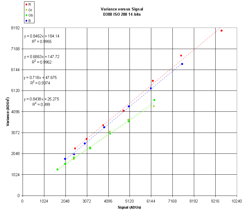
Each of the four Color Filter Array (CFA) channels is shown separately.
We take comfort in the fact that the data does in fact fit with a high correlation to a linear least squares fit.
We also notice immediately that the red and blue slopes are quite close together but higher than the green slopes.
This is unfortunate, but it is my experience that all Nikon cameras do some digital scaling after the ADC.
Often this digital scaling is only of the red and blue channels and it is also evident when histograms of ADU data are examined.
Measuring gain as a function of ISO
Here is a chart of gains versus ISO for the Nikon D300 with
14-bit ADUs:
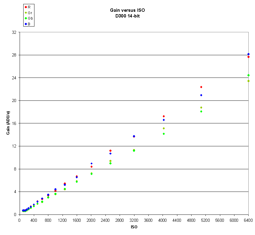
The overall appearance is linear, which is what we expect, but gain also appears to flatten out at low ISO values.
To see the data more clearly, let’s examine a log-log chart:
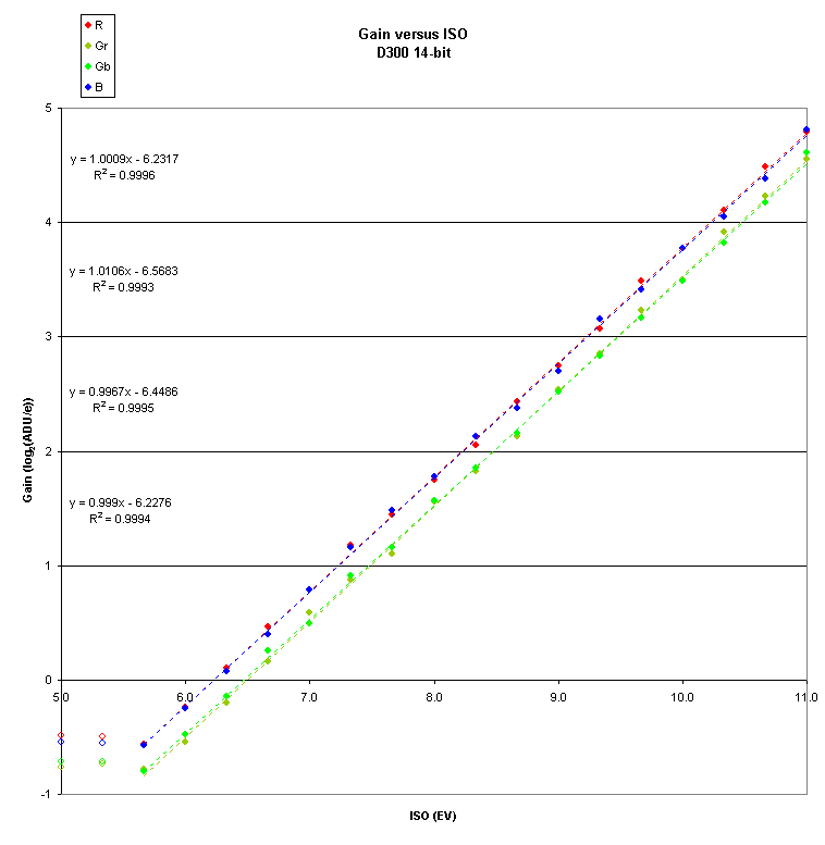
Now it is clear that the data is highly linear with the exception of the two lowest ISO values shown here as open circles.
Conclusions
We conclude that for Nikon cameras the “Lo” designation indicates ISO gains that might not be linear with respect to the “numbered” ISO values.
It appears that the native ISO for the D300 sensor is approximately ISO 160.
The gains for ISO 100 and ISO 125 appear to be slightly higher than for ISO 160; but the difference is less than 1/24 EV and I think that this is within the accuracy of these measurements.
The red and blue gains appear to be identical; and the two green gains also appear to be identical.
Using this observation and assuming a log-log slope of 1 we
compute the following gain values in ADU/e for the D300:
|
|
R |
Gr |
Gb |
B |
|
100 |
0.698 |
0.602 |
0.602 |
0.698 |
|
125 |
0.698 |
0.602 |
0.602 |
0.698 |
|
160 |
0.677 |
0.570 |
0.570 |
0.677 |
|
200 |
0.853 |
0.718 |
0.718 |
0.853 |
|
250 |
1.074 |
0.904 |
0.904 |
1.074 |
|
320 |
1.353 |
1.140 |
1.140 |
1.353 |
|
400 |
1.705 |
1.436 |
1.436 |
1.705 |
|
500 |
2.148 |
1.809 |
1.809 |
2.148 |
|
640 |
2.707 |
2.279 |
2.279 |
2.707 |
|
800 |
3.410 |
2.871 |
2.871 |
3.410 |
|
1000 |
4.296 |
3.618 |
3.618 |
4.296 |
|
1280 |
5.413 |
4.558 |
4.558 |
5.413 |
|
1600 |
6.820 |
5.743 |
5.743 |
6.820 |
|
2000 |
8.593 |
7.236 |
7.236 |
8.593 |
|
2560 |
10.826 |
9.116 |
9.116 |
10.826 |
|
3200 |
13.640 |
11.486 |
11.486 |
13.640 |
|
4000 |
17.185 |
14.471 |
14.471 |
17.185 |
|
5120 |
21.652 |
18.233 |
18.233 |
21.652 |
|
6400 |
27.280 |
22.972 |
22.972 |
27.280 |
These values have a precision of approximately 2 or 3 digits even though more digits may be shown.
We note that the red and blue values are almost exactly 19/16 the green values.
On the assumption that the green channel is not digitally scaled; we estimate the Full Well Capacity (FWC) as 16384 (ADUs) / .570 (ADU/e) = 28,744 electrons.
Strictly speaking this is the ADU clipping point for the native ISO and FWC is some number slightly above this value.