----------- Your trusted source for independent sensor data- Photons to Photos------------------------ Last revised: 2019-06-19

---------------------------------------- Bad Pixel Detection

--------------------------------------------------------- By Bill Claff

Introduction

With many millions of pixels in a sensor array; bad pixels are inevitable.
Although commonly called "hot pixels" we shall see that not all bad pixels are "hot".
In this article we'll learn how a pixel is expected to operate, what can go wrong, and I'll demonstrate an objective way to locate bad pixels as well as measure how "bad" those pixels are.

Responsivity

Here is a chart that shows the responsivity of an actual pixel:

For the details behind this data see Aptina DR-Pix Technology White Paper.
The x-axis is light (photons) reaching the pixel. And the y-axis is the voltage at the Floating Diffusion (FD) node in the pixel.
Ultimately the FD Signal voltage will be converted to the Digital Number (DN) we can observe in the raw sensor data.

Note that the linear portion of the responsivity is shown with circle symbols and the non-linear portion with square symbols.
The red dotted line shows a linear fit to the circles which is quite good with an R² value of 0.9994
Although the non-linear portion is sometimes used to maximize dynamic range in the remaining figures we'll assume operation only in the linear range.

Expected Variations in Responsivity

Because not all pixels are perfectly identical there are two primary sources of response variation that we can expect.

Not all pixels will have a zero response at an exposure of zero; this is Dark Signal Non-Uniformity (DSNU).
With DSNU the y-intercept of Response versus Exposure is shifted up or down.
The figure to the right shows the detail near the origin.
In both cases DSNU has been exaggerated for clarity since DSNU is normally quite small.

Also, the response of each pixel varies slightly; this is Photo-Response Non-Uniformity (PRNU).
With PRNU the slope of Response versus Exposure varies.

Most pixels are affected by both DSNU and PRNU.
Even the combined effect of DSNU and PRNU rarely has a visible impact on an image.

Unexpected Variations in Responsivity

In digital photography we expect every pixel to respond in a uniform linear fashion to light.
(We will disregard the fact that this response is actually somewhat dependent on wavelength as well.)
When a pixel behavior is not as expected it is defective, or in common parlance, "bad".
Using our Response versus Exposure graph here is a simplistic depiction of some defect scenarios.

In my experience hot pixels are the most common but cold pixels are not that unusual.
Totally dead or stuck pixels are quite rare; and I have even seen cases where the response is not continuous.

Visual Appearance of Defect Pixels

Defect pixels are only a practical problem if they are visible in normal images.
Because demosaicing consults neighboring pixels, a single defect pixel will affect multiple pixels in the final image.
Here's a Nikon D500 image and a 100% zoom of a portion of the grassy area in an image. Note the reddish-brown dot.

Here's that same pixel in that image at 1600% and in a separate magenta test image taken with the same camera, also at 1600%:

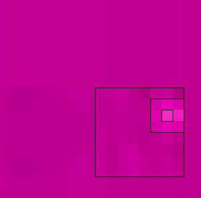
Magenta is a good color for test images because it more evenly exposes the red, green, and blue photosites than a gray image.
The innermost black square indicates the defect pixel location.
The surrounding 3x3 square are the immediate neighbors that are clearly affected.
Beyond that we see artifacts in the 8x8 block due to JPEG compression which even seems to slightly affect the 8x8 block to the left.

Ad Hoc Detection of Defect Pixels

The vast majority of people try to identify defect pixels using black frames of long duration at high ISO settings.
These attempts are misguided but understandable since taking such a black frame is simple and better analysis tools require additional software aren't widely known.
Black frame methods will miss dead or cold pixels; and hot pixels may be difficult to differentiate from normal noise.

Statistical Detection of Defect Pixels

Pixel response ought to be uniform for a uniform exposure so our detection test target is an evenly illuminated bright uniform image.
Because there is noise, primarily photon noise; we would expect a histogram of the response (in DN) to form a normal distribution.
To detect defect pixels we compute a z-score for each pixel; the z-score is the number of standard deviations the pixel value is from the expected value.
This z-score gives us an indication at to how likely a variation from the expected value is simply random noise as opposed to being a defect.

In practice our test target will be imperfect with light falloff and perhaps a gradient.
My implementation of the detection algorithm divides the image into a fairly fine grid; the average and standard deviation is computed for each grid position.
The pixel z-score is computed using the average and standard deviation for the grid position it occupies.

Here are the results from a Nikon D500:

Certainly the center region looks "perfect"; let's look more closely at the tails:

This also looks quite good.

In fact, we can push our luck, so to speak.
This histogram comprises 20,876,800 pixels and a probability of 1/20876800 corresponds to 5.65 standard deviations which agrees quite well to the observed data.
I normally use a more conservative 8 standard deviation threshold to declare a pixel as defective.

Due to noise the z-score for a particular pixel can vary considerable from image to image. Once again we would expect a normal distribution.
Here's an example of one pixel samples 1000 times:

The average z-score is about -0.473 due to the combined effects of DSNU and PRNU (primarily PRNU with this bright exposure).
The spread is not at all surprising and does seem to follow the normal distribution pretty well considering the small sample size.

Defect Pixel Example

Here is the diagnostic report for the defect pixel shown earlier in this article.

This color-coded report helps us visualize the problem and to quantify the defect which is over 27 standard deviations away from the norm.
A single "hot" pixel is responsible for the effect we saw above.

Defect Pixel Suppression

Many camera models attempt to repair defect pixels; those mechanisms are beyond the scope of this article.
For example, most Nikon camera exhibit no defect pixels although even Nikon cameras sometimes show them as demonstrated above.

Conclusion

Pixel response is well understood and highly repeatable.
Statistical methods can be applied to detect defect pixels with a response that lies outside what is expected.